
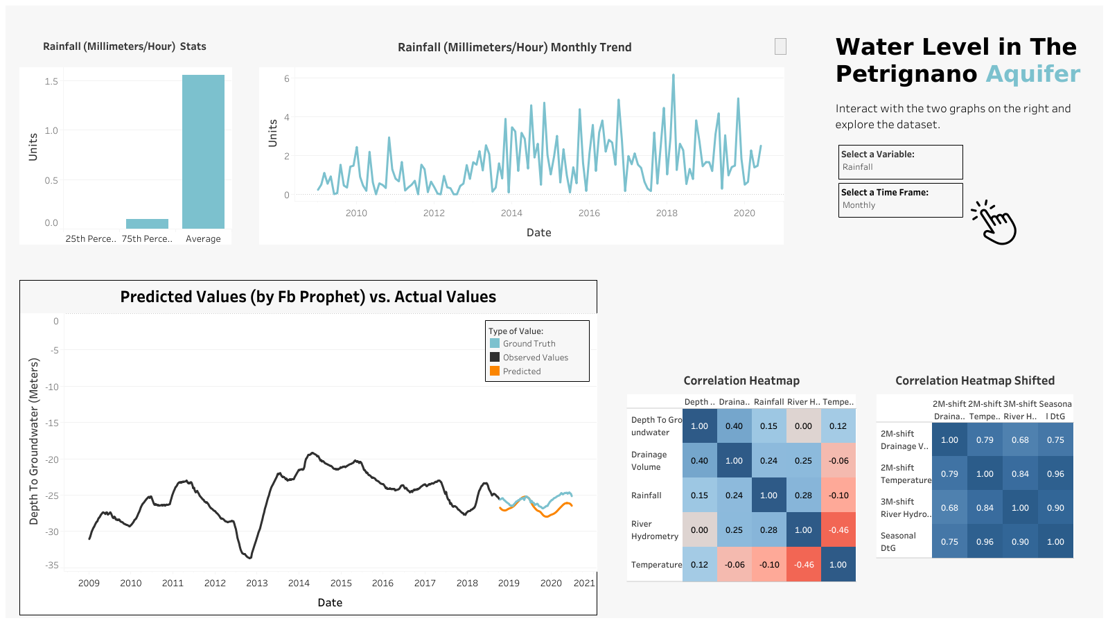
Check the final dashboard here: Tableau Dashboard
In [ ]:
import pandas as pd
import numpy as np
from datetime import datetime, date

import seaborn as sns
import matplotlib.pyplot as plt

from sklearn.metrics import mean_absolute_error, mean_squared_error

import warnings # Supress warnings
warnings.filterwarnings('ignore')
In [ ]:
path = r'C:\Users\matte\OneDrive\Desktop\GitHub\data\Petrignano\Aquifer_Petrignano.csv'
df = pd.read_csv(path)
df.head()
Out[ ]:
| Date | Rainfall_Bastia_Umbra | Depth_to_Groundwater_P24 | Depth_to_Groundwater_P25 | Temperature_Bastia_Umbra | Temperature_Petrignano | Volume_C10_Petrignano | Hydrometry_Fiume_Chiascio_Petrignano | |
|---|---|---|---|---|---|---|---|---|
| 0 | 14/03/2006 | NaN | -22.48 | -22.18 | NaN | NaN | NaN | NaN |
| 1 | 15/03/2006 | NaN | -22.38 | -22.14 | NaN | NaN | NaN | NaN |
| 2 | 16/03/2006 | NaN | -22.25 | -22.04 | NaN | NaN | NaN | NaN |
| 3 | 17/03/2006 | NaN | -22.38 | -22.04 | NaN | NaN | NaN | NaN |
| 4 | 18/03/2006 | NaN | -22.60 | -22.04 | NaN | NaN | NaN | NaN |
In [ ]:
# Remove not usefull columns
df = df[df.Rainfall_Bastia_Umbra.notna()].reset_index(drop=True)
df = df.drop(['Depth_to_Groundwater_P24', 'Temperature_Petrignano'], axis=1)
In [ ]:
# Simplify column names
df.columns = ['date', 'rainfall', 'depth_to_groundwater', 'temperature', 'drainage_volume', 'river_hydrometry']
In [ ]:
df.info()
<class 'pandas.core.frame.DataFrame'>
RangeIndex: 4199 entries, 0 to 4198
Data columns (total 6 columns):
 #   Column                Non-Null Count  Dtype
---  ------                --------------  -----
 0   date                  4199 non-null   object
 1   rainfall              4199 non-null   float64
 2   depth_to_groundwater  4172 non-null   float64
 3   temperature           4199 non-null   float64
 4   drainage_volume       4198 non-null   float64
 5   river_hydrometry      4199 non-null   float64
dtypes: float64(5), object(1)
memory usage: 197.0+ KB
Data cleaning
In [ ]:
# Parse object type to datetime type
df['date'] = pd.to_datetime(df['date'], format = '%d/%m/%Y')
df.head()
Out[ ]:
| date | rainfall | depth_to_groundwater | temperature | drainage_volume | river_hydrometry | |
|---|---|---|---|---|---|---|
| 0 | 2009-01-01 | 0.0 | -31.14 | 5.2 | -24530.688 | 2.4 |
| 1 | 2009-01-02 | 0.0 | -31.11 | 2.3 | -28785.888 | 2.5 |
| 2 | 2009-01-03 | 0.0 | -31.07 | 4.4 | -25766.208 | 2.4 |
| 3 | 2009-01-04 | 0.0 | -31.05 | 0.8 | -27919.296 | 2.4 |
| 4 | 2009-01-05 | 0.0 | -31.01 | -1.9 | -29854.656 | 2.3 |
In [ ]:
df.isna().sum()
Out[ ]:
date                     0
rainfall                 0
depth_to_groundwater    27
temperature              0
drainage_volume          1
river_hydrometry         0
dtype: int64
In [ ]:
fig, ax = plt.subplots(nrows=5, ncols=1, figsize=(15, 25))

for i, column in enumerate(df.drop('date', axis=1).columns):
    # For now I handle missing value with fillna
    sns.lineplot(x=df['date'], y=df[column].fillna(method='ffill'), ax=ax[i], color='steelblue')
    ax[i].set_title(column, fontsize=17)
    ax[i].set_ylabel(column, fontsize=17)

    ax[i].set_xlim([date(2009, 1, 1), date(2020, 6, 30)])

I see no reasons why the river_hydrometry would be 0 just before 2016. This is likely a bias in the data, so I'll convert values == 0 to np.nan.
In [ ]:
df['river_hydrometry_back_up'] = df['river_hydrometry'].copy()
df.loc[df['river_hydrometry']==0, 'river_hydrometry'] = np.nan

# Fill nan values with interpolate
df['hydro_fill'] = df['river_hydrometry'].interpolate()

# This is for the next visualization
df.loc[df['river_hydrometry'].notna(), 'hydro_fill'] = np.nan
In [ ]:
fig, ax = plt.subplots(figsize=(12, 5))

sns.lineplot(x=df['date'], y=df['river_hydrometry'], color='steelblue',
             label='original', ax=ax)
sns.lineplot(x=df['date'], y=df['hydro_fill'], color='orange',
             label='interpolate', ax=ax)
ax.set_xlim([date(2012, 5, 1), date(2016, 10, 1)])
plt.show()

In [ ]:
# interpolate in this case is quite good, so I'll use it for each of the columns

df.loc[df['depth_to_groundwater']==0, 'depth_to_groundwater'] = np.nan
df.loc[df['river_hydrometry']==0, 'river_hydrometry'] = np.nan

df['river_hydrometry'] = df['river_hydrometry'].interpolate()
df['drainage_volume'] = df['drainage_volume'].interpolate()
df['depth_to_groundwater'] = df['depth_to_groundwater'].interpolate()
df.drop(columns=['hydro_fill', 'river_hydrometry_back_up'], inplace=True)

df.head()
Out[ ]:
| date | rainfall | depth_to_groundwater | temperature | drainage_volume | river_hydrometry | |
|---|---|---|---|---|---|---|
| 0 | 2009-01-01 | 0.0 | -31.14 | 5.2 | -24530.688 | 2.4 |
| 1 | 2009-01-02 | 0.0 | -31.11 | 2.3 | -28785.888 | 2.5 |
| 2 | 2009-01-03 | 0.0 | -31.07 | 4.4 | -25766.208 | 2.4 |
| 3 | 2009-01-04 | 0.0 | -31.05 | 0.8 | -27919.296 | 2.4 |
| 4 | 2009-01-05 | 0.0 | -31.01 | -1.9 | -29854.656 | 2.3 |
In [ ]:
df.to_csv(r'C:\Users\matte\OneDrive\Desktop\GitHub\data\Petrignano\4 tableau\daily_values.csv',
          index=False)
Resampling
It's almost impossible to predict the depth_to_groundwater daily. There are just too many random factors that influence the daily level. Hence, we'll resemple the data.
Each row will be the weekly average.
In [ ]:
fig, ax = plt.subplots(ncols=1, nrows=3, sharex=True, figsize=(16,12))

sns.lineplot(x=df['date'], y=df['temperature'], color='steelblue', ax=ax[0])
ax[0].set_title('Daily Temperature', fontsize=14)

weekly_temp = df[['date','temperature']].resample('7D', on='date').mean().reset_index(drop=False)
sns.lineplot(x=weekly_temp['date'], y=weekly_temp['temperature'], color='steelblue', ax=ax[1])
ax[1].set_title('Weekly Temperature', fontsize=14)

monthly_temp = df[['date','temperature']].resample('1M', on='date').mean().reset_index(drop=False)
sns.lineplot(x=monthly_temp['date'], y=monthly_temp['temperature'], color='steelblue', ax=ax[2])
ax[2].set_title('Monthly Temperature', fontsize=14)

for i in range(3):
    ax[i].set_xlim([date(2009, 1, 1), date(2020, 6, 30)])
plt.show()

In [ ]:
# I'll downsample to weekly so it's easier to predict

downsample = df[['date',
                 'depth_to_groundwater',
                 'temperature',
                 'drainage_volume',
                 'river_hydrometry',
                 'rainfall'
                ]].resample('7D', on='date').mean().reset_index(drop=False)

df = downsample.copy()
Data Preprocessing
In [ ]:
df['year'] = df['date'].dt.year
df['month'] = df['date'].dt.month
df['day'] = df['date'].dt.day
df['day_of_year'] = df['date'].dt.dayofyear
df['quarter'] = df['date'].dt.quarter
df['season'] = df['month'] % 12 // 3 + 1

df[['date', 'year', 'month', 'day', 'day_of_year', 'quarter','season']].head()
Out[ ]:
| date | year | month | day | day_of_year | quarter | season | |
|---|---|---|---|---|---|---|---|
| 0 | 2009-01-01 | 2009 | 1 | 1 | 1 | 1 | 1 |
| 1 | 2009-01-08 | 2009 | 1 | 8 | 8 | 1 | 1 |
| 2 | 2009-01-15 | 2009 | 1 | 15 | 15 | 1 | 1 |
| 3 | 2009-01-22 | 2009 | 1 | 22 | 22 | 1 | 1 |
| 4 | 2009-01-29 | 2009 | 1 | 29 | 29 | 1 | 1 |
In [ ]:
# encoding cyclical features

df['month_sin'] = np.sin(2*np.pi*df['month']/12)
df['month_cos'] = np.cos(2*np.pi*df['month']/12)
In [ ]:
# timeseries decomposition

from statsmodels.tsa.seasonal import seasonal_decompose

to_decompose = [
    'rainfall', 'temperature', 'drainage_volume',
    'river_hydrometry', 'depth_to_groundwater'
]

for column in to_decompose:
    decomp = seasonal_decompose(df[column], period=52, model='additive', extrapolate_trend='freq')
    df[f"{column}_trend"] = decomp.trend
    df[f"{column}_seasonal"] = decomp.seasonal
In [ ]:
df.head()
Out[ ]:
| date | depth_to_groundwater | temperature | drainage_volume | river_hydrometry | rainfall | year | month | day | day_of_year | ... | rainfall_trend | rainfall_seasonal | temperature_trend | temperature_seasonal | drainage_volume_trend | drainage_volume_seasonal | river_hydrometry_trend | river_hydrometry_seasonal | depth_to_groundwater_trend | depth_to_groundwater_seasonal | |
|---|---|---|---|---|---|---|---|---|---|---|---|---|---|---|---|---|---|---|---|---|---|
| 0 | 2009-01-01 | -31.048571 | 1.657143 | -28164.918857 | 2.371429 | 0.000000 | 2009 | 1 | 1 | 1 | ... | 0.806294 | 0.688948 | 15.329959 | -9.739920 | -32404.467037 | 1465.324852 | 2.164913 | 0.295306 | -29.571657 | -0.643767 |
| 1 | 2009-01-08 | -30.784286 | 4.571429 | -29755.789714 | 2.314286 | 0.285714 | 2009 | 1 | 8 | 8 | ... | 0.809093 | -0.728055 | 15.312814 | -9.838787 | -32374.371773 | 852.060183 | 2.167252 | 0.274285 | -29.535110 | -0.572078 |
| 2 | 2009-01-15 | -30.420000 | 7.528571 | -25463.190857 | 2.300000 | 0.028571 | 2009 | 1 | 15 | 15 | ... | 0.811892 | -0.717139 | 15.295668 | -10.002955 | -32344.276508 | 683.230538 | 2.169592 | 0.193182 | -29.498564 | -0.484281 |
| 3 | 2009-01-22 | -30.018571 | 6.214286 | -23854.422857 | 2.500000 | 0.585714 | 2009 | 1 | 22 | 22 | ... | 0.814691 | 0.493481 | 15.278522 | -9.973161 | -32314.181244 | 355.982452 | 2.171931 | 0.219752 | -29.462017 | -0.417712 |
| 4 | 2009-01-29 | -29.790000 | 5.771429 | -25210.532571 | 2.500000 | 1.414286 | 2009 | 1 | 29 | 29 | ... | 0.817490 | -0.556499 | 15.261377 | -10.246938 | -32284.085980 | 65.586895 | 2.174270 | 0.240426 | -29.425470 | -0.362900 |
5 rows × 24 columns
In [ ]:
fig, ax = plt.subplots(ncols=1, nrows=4, sharex=True, figsize=(16,8))
col = 'depth_to_groundwater'

res = seasonal_decompose(df[col], period=52, model='additive',
                         extrapolate_trend = 'freq')

ax[0].set_title(f'{col} Observed')
res.observed.plot(ax= ax[0], legend=False, color='steelblue')

ax[1].set_title(f'{col} Trend')
res.trend.plot(ax=ax[1], legend=False, color='steelblue')

ax[2].set_title(f'{col} Seasonal')
res.seasonal.plot(ax=ax[2], legend=False, color='steelblue')

ax[3].set_title(f'{col} Residual')
res.resid.plot(ax=ax[3], legend=False, color='steelblue')

plt.show()

In [ ]:
# Temperature and rainfall don't immidiately influence the water level.
# So we'll shift them.

for column in to_decompose:
    df[f'{column}_seasonal_shift_b_2m'] = df[f'{column}_seasonal'].shift(-2 * 4) #4=weeks_in_month
    df[f'{column}_seasonal_shift_b_1m'] = df[f'{column}_seasonal'].shift(-1 * 4)
    df[f'{column}_seasonal_shift_1m'] = df[f'{column}_seasonal'].shift(1 * 4)
    df[f'{column}_seasonal_shift_2m'] = df[f'{column}_seasonal'].shift(2 * 4)
    df[f'{column}_seasonal_shift_3m'] = df[f'{column}_seasonal'].shift(3 * 4)
Correlation
In [ ]:
f, ax = plt.subplots(nrows=1, ncols=2, figsize=(16, 8))

corrmat = df[to_decompose].corr()

sns.heatmap(corrmat, annot=True, vmin=-1, vmax=1, cmap='coolwarm_r', ax=ax[0])
ax[0].set_title('Correlation Matrix of Core Features', fontsize=16)

shifted_cols = [
    'depth_to_groundwater_seasonal',
    'temperature_seasonal_shift_b_2m',
    'drainage_volume_seasonal_shift_2m',
    'river_hydrometry_seasonal_shift_3m'
]
corrmat = df[shifted_cols].corr()

sns.heatmap(corrmat, annot=True, vmin=-1, vmax=1, cmap='coolwarm_r', ax=ax[1])
ax[1].set_title('Correlation Matrix of Lagged Features', fontsize=16)


plt.tight_layout()
plt.show()

In [ ]:
df[to_decompose].corr().to_csv(r'C:\Users\matte\OneDrive\Desktop\GitHub\data\Petrignano\4 tableau\corr_matrix_normal.csv')
df[to_decompose].corr()
Out[ ]:
| rainfall | temperature | drainage_volume | river_hydrometry | depth_to_groundwater | |
|---|---|---|---|---|---|
| rainfall | 1.000000 | -0.103933 | 0.242981 | 0.281407 | 0.148775 |
| temperature | -0.103933 | 1.000000 | -0.056979 | -0.457835 | 0.115366 |
| drainage_volume | 0.242981 | -0.056979 | 1.000000 | 0.247127 | 0.402501 |
| river_hydrometry | 0.281407 | -0.457835 | 0.247127 | 1.000000 | 0.002796 |
| depth_to_groundwater | 0.148775 | 0.115366 | 0.402501 | 0.002796 | 1.000000 |
In [ ]:
df[shifted_cols].corr().to_csv(r'C:\Users\matte\OneDrive\Desktop\GitHub\data\Petrignano\4 tableau\corr_matrix_shift.csv')
df[shifted_cols].corr()
Out[ ]:
| depth_to_groundwater_seasonal | temperature_seasonal_shift_b_2m | drainage_volume_seasonal_shift_2m | river_hydrometry_seasonal_shift_3m | |
|---|---|---|---|---|
| depth_to_groundwater_seasonal | 1.000000 | 0.961653 | 0.754727 | 0.899721 |
| temperature_seasonal_shift_b_2m | 0.961653 | 1.000000 | 0.785226 | 0.839125 |
| drainage_volume_seasonal_shift_2m | 0.754727 | 0.785226 | 1.000000 | 0.675689 |
| river_hydrometry_seasonal_shift_3m | 0.899721 | 0.839125 | 0.675689 | 1.000000 |
Machine Learning Prediction
In [ ]:
train_size = int(0.85 * len(df))
test_size = len(df) - train_size

univariate_df = df[['date', 'depth_to_groundwater']].copy()
univariate_df.columns = ['ds', 'y']

train = univariate_df.iloc[:train_size, :]

x_train, y_train = pd.DataFrame(univariate_df.iloc[:train_size, 0]), pd.DataFrame(univariate_df.iloc[:train_size, 1])
x_valid, y_valid = pd.DataFrame(univariate_df.iloc[train_size:, 0]), pd.DataFrame(univariate_df.iloc[train_size:, 1])

print(len(train), len(x_valid))
510 90
In [ ]:
from prophet import Prophet

# Train the model
model = Prophet()
model.fit(train)

y_hat = model.predict(x_valid)

# Calcuate metrics
score_mae = mean_absolute_error(y_valid, y_hat.tail(test_size)['yhat'])
score_rmse = np.sqrt(mean_squared_error(y_valid, y_hat.tail(test_size)['yhat']))

print(f'RMSE: {score_rmse}')
14:37:30 - cmdstanpy - INFO - Chain [1] start processing
14:37:30 - cmdstanpy - INFO - Chain [1] done processing
RMSE: 1.1969132721330753
In [ ]:
ml_predict = pd.merge(df[['date', 'depth_to_groundwater']], y_hat[['ds', 'yhat']],
         how='outer', left_on='date', right_on='ds')

ml_predict.drop(columns='ds', inplace=True)
ml_predict.tail()
Out[ ]:
| date | depth_to_groundwater | yhat | |
|---|---|---|---|
| 595 | 2020-05-28 | -24.697143 | -26.122581 |
| 596 | 2020-06-04 | -24.638571 | -26.148812 |
| 597 | 2020-06-11 | -24.751429 | -26.203053 |
| 598 | 2020-06-18 | -24.822857 | -26.305481 |
| 599 | 2020-06-25 | -25.145000 | -26.468179 |
In [ ]:
ml_predict.to_csv(r'C:\Users\matte\OneDrive\Desktop\GitHub\data\Petrignano\4 tableau\predictions.csv',
             index=False)
In [ ]:
fig, ax = plt.subplots(figsize=(12,6))

model.plot(y_hat, ax=ax)
sns.lineplot(x=x_valid['ds'], y=y_valid['y'], ax=ax, color='orange', label='Ground truth')

ax.set_title(f'Prediction \n MAE: {score_mae:.2f}, RMSE: {score_rmse:.2f}', fontsize=14)
ax.set_xlabel(xlabel='Date', fontsize=14)
ax.set_ylabel(ylabel='Depth to Groundwater', fontsize=14)

plt.show()
